
Gradient boosting with LightGBM
- Lesson 15
- 45 min
- Module 5: Machine learning forecasters
Where we are
In the last lesson, we built forecasting features by hand and fit a linear regression. It used the promotion flag, but it added the same number of units for every product. In this lesson, we train one LightGBM model for all products with mlforecast, forecast many days ahead in two ways, and avoid the leakage traps that rolling features hide. Think first of a golfer on the green.
Lesson 15 of 27 · Forecasting and Time Series: Predict What Comes NextGradient boosting with LightGBM
1. Forecasts serve decisions
2. Read a time series
3. Baselines and honest testing
4. Statistical forecasters
5. Machine learning forecasters
6. Hard series and many series
7. Uncertainty and the decision
8. Run a forecast in production
What you will be able to do
Train one gradient boosting model for all products, forecast 14 days ahead without breaking the gap, and recognise a rolling feature that leaks the future. LightGBM gives the lowest order cost of the course table, if you set it up honestly.
NotebookDo this lesson in a notebook
The notebook has every code cell, task and check of this lesson. It trains LightGBM, backtests three set-ups and finds the leak in a rolling mean. Its setup cells install the packages and download the Larkfield data, so it needs no local setup. About 45 minutes, of which 2 to 3 minutes of waiting.
Colab and Kaggle open your own copy. They need a free Google or Kaggle account. Stuck? See the solution notebook.
Before you startWhat to know and to have ready
What you need to know
- Lags, rolling means, known future inputs and a global model, from Forecasting as regression.
- Decision trees and gradient boosting: see Decision trees and Ensembles in the machine learning course. This lesson recalls the idea briefly.
- The cost column of the backtest table, from Measure the error that matters.
What you need on your computer
Nothing: the notebook runs in Colab or Kaggle. Its first cell installs mlforecast 1.1.0 and LightGBM 4.7.0.
Tested with Python 3.12, pandas 2.3.3, mlforecast 1.1.0 and LightGBM 4.7.0, in Jupyter on macOS.
A golfer on the green
Section titled “A golfer on the green”A golfer is on the green, 10 metres from the hole. The first putt stops 2 metres short. The second putt aims only at the 2 metres that are left. It stops 30 centimetres past the hole, and the third putt fixes those 30 centimetres.
Each putt is small and imperfect. But each one corrects what the putts before it left. Together they reach the hole.
The problem: one fixed number for every product
Section titled “The problem: one fixed number for every product”The global linear regression of the last lesson used the promotion flag. It learned one weight for it: “on promotion, add w units”. The same w for every product.
Here is a tiny constructed example. Two products, each seen on a normal day and on a promotion day:
| Product | On promotion | Units sold | Linear model | Miss |
|---|---|---|---|---|
| slow | no | 4 | 0 | 4 |
| slow | yes | 8 | 12 | −4 |
| fast | no | 20 | 24 | −4 |
| fast | yes | 40 | 36 | 4 |
A promotion doubles the sales of both products: +4 for the slow one, +20 for the fast one. The best linear model with the columns “fast” and “on promotion” is: units = 24 × fast + 12 × promotion. Its 12 units are too many for the slow product and too few for the fast one. No weights fix this, because the effect of a promotion depends on the product. Two features that act together like this have an interaction.
Larkfield’s promotions work like this. Their median uplift is ×1.87 (from Calendars, holidays and events): a multiplication, not an addition.
The idea: many small trees, each fixing the last errors
Section titled “The idea: many small trees, each fixing the last errors”A decision tree predicts by asking yes-or-no questions: “Is the product a fast seller? Is it on promotion?” Each answer leads to a leaf with a number. A tree can ask about the promotion after it asked about the product, so it can give a different uplift to each kind of product.
One small tree is a weak forecaster. Gradient boosting builds many of them, like the golfer’s putts:
- Start with one number for every row: the mean.
- Compute the errors that are left.
- Fit a small tree that predicts those errors.
- Add a small step of that tree to the forecast.
- Repeat, hundreds of times.
The name says what it does. Boosting: weak models, one after the other, become a strong one. Gradient: each new tree follows the direction that reduces the error most. LightGBM is a library that does this fast on large tables. The machine learning course explains it in depth in Ensembles.
A tiny worked example: two trees
Section titled “A tiny worked example: two trees”The same four rows. Real libraries take very small steps (here 0.05) and grow many trees. This example takes full steps, so that two trees are enough.
| Product | Promotion | Sold | Start (mean) | Error left | Tree 1: fast? | After tree 1 | Error left | Tree 2: fast? then promotion? | After tree 2 |
|---|---|---|---|---|---|---|---|---|---|
| slow | no | 4 | 18 | −14 | −12 | 6 | −2 | −2 | 4 |
| slow | yes | 8 | 18 | −10 | −12 | 6 | 2 | +2 | 8 |
| fast | no | 20 | 18 | 2 | +12 | 30 | −10 | −10 | 20 |
| fast | yes | 40 | 18 | 22 | +12 | 30 | 10 | +10 | 40 |
Follow the slow product on promotion, the second row. The start is the mean of the four rows: (4 + 8 + 20 + 40) ÷ 4 = 18. Tree 1 asks one question, “fast seller?”, and predicts the mean error of each group: −12 for the slow rows. So the forecast becomes 18 − 12 = 6. The error left is 8 − 6 = 2. Tree 2 asks two questions, “fast?” then “on promotion?”, and predicts +2 for this leaf. The forecast is 6 + 2 = 8.
Tree 2 gives +2 to the slow product on promotion and +10 to the fast one: the interaction that the linear model could not learn. On real data, the many small steps keep the model from learning the noise.
Larkfield: one LightGBM model for all products
Section titled “Larkfield: one LightGBM model for all products”Priya trains LightGBM with mlforecast, with the inputs of the course table. They are the lags of 1, 7, 14 and 28 days and the means of the last 7 and 28 days. One more input is the mean of lags 7 to 10: the 4 days that end a week back. The calendar adds the weekday, the month and the day of the year. The known inputs are the price, the promotion flag and three holiday flags.
import lightgbm as lgbfrom mlforecast import MLForecastfrom mlforecast.lag_transforms import RollingMean
LGB = dict(n_estimators=400, learning_rate=0.05, num_leaves=63, min_child_samples=20, subsample=0.8,           subsample_freq=1, colsample_bytree=0.8, random_state=35, n_jobs=2, verbose=-1)
def make_model(lags, lag_transforms):    return MLForecast(models={"lgbm": lgb.LGBMRegressor(**LGB)}, freq="D", lags=lags, lag_transforms=lag_transforms,                      date_features=["dayofweek", "month", "dayofyear"], num_threads=1)
RECURSIVE = dict(lags=[1, 7, 14, 28], lag_transforms={1: [RollingMean(7), RollingMean(28)], 7: [RollingMean(4)]})
n_estimators=400 is the number of trees. learning_rate=0.05 is the size of each step. num_leaves=63 limits the size of each tree. These are the settings of the course table, not tuned values.
At the 13 origins of the course backtest, the notebook prints:
method horizon MASE WAPE % bias % pinball fit s cost $LightGBM, recursive 14 0.816 40.7 0.7 12.54 14749LightGBM beats ETS (41.3%) and both linear regressions (41.7% and 42.6%) on WAPE, and its order costs 14,749 dollars against 16,578 for ETS. On the 154 promotion days, its bias is +5.2%. ETS was −43.5% there.
The parasol in the backtest
Section titled “The parasol in the backtest”The explorer has the methods that you have met so far. Move the origin and compare LightGBM with ETS and the baselines on the parasol.
Explore
LightGBM on the parasol
Predict first: Over all 13 origins, does LightGBM beat ETS on the parasol, and by how much?
- Sold in the 14 days
- 101
- Forecast for the 14 days
- 114
- WAPE at this origin
- 44.8%
- WAPE, all 13 origins
- 49.3%
At the origin 8 Jun 2025, LightGBM (recursive) forecasts 114 units for the next 14 days. 101 were sold. Its WAPE here is 44.8%: it is too high. Over all 13 origins, LightGBM (recursive) has a WAPE of 49.3%: number 1 of 5 methods. It beats the baseline, seasonal naive (66.1%).
- Units sold
- Forecast of the chosen method
- Baseline: seasonal naive
Show every method, ranked
| Rank | Method | Family | WAPE at this origin | WAPE, all 13 origins |
|---|---|---|---|---|
| 1 | LightGBM (recursive) | machine learning | 44.8% | 49.3% |
| 2 | AutoARIMA | statistical | 51.7% | 62.6% |
| 3 | moving average (28 days) | baseline | 101.3% | 64.9% |
| 4 | ETS | statistical | 45.5% | 65.1% |
| 5 | seasonal naive | baseline | 74.3% | 66.1% |
Text description of the explorer
The explorer shows the parasol’s daily sales: the four weeks before the chosen origin (grey line) and the 14 days after it (grey dots). It adds the chosen method’s forecast (blue) and the seasonal naive forecast (dashed orange). The controls choose the origin (13 April 2025 to 15 March 2026) and one of five methods. At the origin of 8 June 2025, 101 parasols were sold; LightGBM forecast 114 (WAPE 44.8% at this origin) and ETS 92 (45.5%). Over all 13 origins, the WAPE of each method is: LightGBM (recursive) 49.3%, AutoARIMA 62.6%, moving average (28 days) 64.9%, ETS 65.1% and seasonal naive 66.1%.
On the parasol, LightGBM wins clearly. Across the 50 products, the lead is much smaller, and ETS still wins on 21. The last lesson of this module looks at that.
Many days ahead: recursive or direct
Section titled “Many days ahead: recursive or direct”Kenji’s order covers 14 days. The model above uses lag1, but on day 5 of the order, “yesterday” has not happened yet. There are three honest answers.

Text description of the diagram
The top panel, recursive, shows a box “known up to Sunday”, then one model that feeds day 1, day 2, day 3 and day 14. Arrows say that each forecast becomes the next day’s lag 1, so an error on day 1 can pile up. The bottom panel, direct, shows the same days, each with its own model, model 1 to model 14. Each model sees only what is known on Sunday.
- Recursive (mlforecast’s default): one model. Its forecast for day 1 becomes
lag1for day 2, and so on. It is fast, but an error on day 1 is carried into day 2. - Lags of 14 days and more: one model with only inputs that are at least 14 days old. Nothing needs to be filled in, but the model never sees the last two weeks.
- Direct:
max_horizon=14trains 14 models. The model for day 5 learns from rows where the inputs are 5 days older than the target. No forecast is fed back, but the fit takes much longer.
The course table has all three:
- Statistical method
- Machine learning
Text description of the chart
Three panels. WAPE: ETS 41.3%, LightGBM recursive 40.7%, lags of 14 days and more 40.9%, direct 40.7%. Cost of the 14-day order: ETS 16,578 dollars, recursive 14,749, lags of 14 days and more 14,629, direct 13,711. Fit time for the 13 origins: ETS about 46 seconds, recursive about 16, lags of 14 days and more about 12, direct about 156.
The three have almost the same WAPE, but their costs differ. The direct forecast costs 1,038 dollars less per order than the recursive one.
Be careful with small tests. To save time, the notebook runs the direct forecast at the last 4 origins only. There, it is the most expensive of the three:
method horizon MASE WAPE % bias % pinball fit s cost $lags >= 14, last 4 cut-offs 14 0.652 38.9 -1.4 12.49 9174 recursive, last 4 cut-offs 14 0.682 41.9 0.2 12.54 9756 direct, last 4 cut-offs 14 0.696 42.0 2.7 93.53 9926(The fit s of the first two rows is the time of all 13 origins.) Four origins are four winter and early-spring windows, and the order of the methods changes between origins. Compare them on all 13.
Leakage hides in rolling features
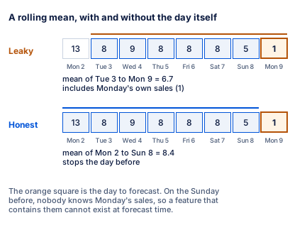
Section titled “Leakage hides in rolling features”A rolling mean is LightGBM’s most useful feature, as the next section shows. It is also the easiest one to make wrong.
Text description of the diagram
Two rows show the parasols sold from Monday 2 to Monday 9 June 2025: 13, 8, 9, 8, 8, 8, 5 and 1. Monday 9, in orange, is the day to forecast. In the leaky row, the window covers Tuesday 3 to Monday 9, so its mean, 6.7, includes Monday’s own sale of 1. In the honest row, the window covers Monday 2 to Sunday 8, and its mean is 8.4.
s.rolling(7).mean() in pandas includes the current row. Tomás computes it on the whole series before the backtest and gives it to LightGBM, with the weekday and the promotion flag. In the backtest:
| Method | MASE | WAPE % | Cost $ per order |
|---|---|---|---|
| LightGBM with the leaky rolling mean | 0.671 | 33.5 | 4,899 |
| LightGBM, recursive (honest) | 0.816 | 40.7 | 14,749 |
The leaky model has a third of the honest model’s cost, and that is the warning sign. The model has learned to copy an input that will not exist in the order week.
mlforecast avoids this trap: lag_transforms={1: [RollingMean(7)]} computes the mean from lag 1, so it stops the day before. When you write a feature in pandas, shift first, then roll.
What the model used: feature importance
Section titled “What the model used: feature importance”LightGBM can say how much each feature helped. The gain of a feature is how much the splits on it reduced the error, added up over all trees. Here is the share of each feature in the model trained at the last origin:
Text description of the chart
The top 10 features by share of the gain: mean of the last 7 days 52.4%, mean of the last 28 days 22.5%, yesterday (lag 1) 6.7%, day of the year 4.3%, mean of the same weekday, 4 weeks 4.1%, lag 28 1.8%, lag 7 1.8%, lag 14 1.8%, weekday 1.5%, price 1.2%.
The model mostly asks “how much has this product sold lately?”, then adjusts. Tomás sees no promotion flag in the top 10 and concludes: “Promotions don’t matter.” That is wrong. Promotion days are rare, so splits on them reduce the total error less, even though they matter a lot on those days. Importance tells you what the model used, not what causes sales. The machine learning course explains this limit in Explain predictions.
When to use LightGBM, and what it costs
Section titled “When to use LightGBM, and what it costs”Use a global gradient boosting model when you have many related series and known future inputs. It is strongest when effects interact, such as a promotion that multiplies sales.
Its costs:
- Settings. The number of trees, the step size and the tree size change the result. Tuning them on the backtest makes the score look better than it will be, as Test like the future explained (“many looks”).
- Fit time. Seconds for the recursive model, minutes for the direct one, at every refit.
- No range. LightGBM gives one number per day. Module 7 adds a range.
- No values beyond what it has seen. A tree cannot forecast higher than its highest leaf. If a product grows to sales it never had before, ETS can follow the trend; a tree cannot.
- Trust. Kenji can read an ETS forecast as “recent level plus the weekly pattern”. A model of 400 trees is harder to explain.
Common mistake
A rolling mean that includes the day
Symptom: a new LightGBM model has a WAPE of 33.5% and an order cost of 4,899 dollars. The honest model has 40.7% and 14,749.
Cause: its rolling mean was computed with rolling(7) on the whole series before the backtest. Each day’s feature contains that day’s sales, which are unknown at forecast time.
Fix: build rolling features from lags (shift first, then rolling), or with mlforecast’s lag_transforms. Recompute the features inside the backtest, from each origin’s training data only.
Consequence in AI work: a leaky model wins every backtest and then fails in production. When a model beats every other method by a wide margin, look for leakage before you celebrate.
Guided practice: LightGBM in the notebook
Section titled “Guided practice: LightGBM in the notebook”- Open the notebook from the box Do this lesson in a notebook at the top of this page.
- Run the setup cells and the helper cell. The data cell ends with the
Ready:line. - In section 1, predict which feature LightGBM uses most. Then run the cell. You see
rolling_mean_lag1_window_size7first, with 52.4. - In section 2, predict if LightGBM beats ETS. Then run the backtest. You see WAPE % 40.7 and cost 14749.
- In section 3, run the three set-ups (about a minute). You see the lags of 14 days and more with WAPE % 40.9, then three rows for the last 4 origins.
- In section 4, predict if the leaky model looks better or worse. Then run it. You see WAPE % 33.5.
- In section 5, write your answer in the Your turn cell, then run the check cell.
Your turn: LightGBM on promotion days
Section titled “Your turn: LightGBM on promotion days”ETS missed 43.5% of the units on the 154 promotion days. Before you run anything, predict: is LightGBM too high or too low on those days? In the notebook, section 5, keep the promotion days of fc_rec. Compute their bias in % and put it in promo_bias_lgbm.
Show the answer
p = fc_rec.merge(sales[["unique_id", "ds", "on_promotion"]], on=["unique_id", "ds"])p = p[p["on_promotion"] == 1]promo_bias_lgbm = round(float(100 * (p["yhat"].sum() - p["y"].sum()) / p["y"].sum()), 1)print(promo_bias_lgbm, "% on", len(p), "promotion days")5.2 % on 154 promotion daysLightGBM is 5.2% too high on the promotion days, close to the global linear regression (+5.9%) and far from ETS (−43.5%). It sees the promotion flag. On the other days, it is only 0.5% too high.
Knowledge check
Section titled “Knowledge check”Check your understanding
Explain with the tiny example why a linear model cannot learn a promotion that doubles sales, and how two boosted trees can.
Show the answer
The slow product sells 4, or 8 on promotion; the fast one sells 20, or 40. The promotion adds 4 units to one and 20 to the other. A linear model has one weight for “on promotion”, so it adds the same number to both. It adds 12 units: too many for the slow product and too few for the fast one. Gradient boosting starts from the mean (18) and adds trees that predict the errors left. Tree 1 asks “fast seller?” (−12 or +12). Tree 2 asks “fast?” then “on promotion?” and gives +2 to the slow product on promotion and +10 to the fast one. A tree can give each kind of product its own uplift.
Does your answer have the main points of ours?
Sign in and enroll in the course to save your answers. Every check counts toward the certificate.
Check your understanding
Name the three ways to forecast 14 days ahead with LightGBM, and give one advantage and one cost of the direct forecast, with Larkfield's numbers.
Show the answer
Recursive: one model, which uses its own forecasts as lags for the next days. Lags of 14 days and more: one model with inputs that are all known for the whole order. Direct: one model per day ahead (14 models), each using only what is known at the origin. The direct forecast had the lowest order cost of the course table, 13,711 dollars against 14,749 for the recursive one. It cost about ten times the fit time (about 156 seconds against 16 for the 13 origins). And at the last 4 origins alone, it was the most expensive of the three, so a small test can mislead.
Does your answer have the main points of ours?
Sign in and enroll in the course to save your answers. Every check counts toward the certificate.
Check your understanding
Predict: a colleague's new feature brings LightGBM's WAPE from 40.7% to 33.5%. What do you check first, and how?
Show the answer
Check for leakage first: a jump that large from one feature is the sign of a feature that contains the target. Look at how the feature is computed. A rolling mean with rolling(7) on the whole series, without a shift, includes the day itself. Recompute it from lags (shift, then roll) inside the backtest, from the training data of each origin. On Larkfield, the leaky rolling mean gave 33.5% and an order cost of 4,899 dollars. Without the leak, the model is back at 40.7% and 14,749.
Does your answer have the main points of ours?
Sign in and enroll in the course to save your answers. Every check counts toward the certificate.
Recap
- Gradient boosting adds many small decision trees; each one predicts the errors that the trees before it left. Trees learn interactions, such as a promotion that doubles sales.
- One global LightGBM model for the 50 products: WAPE 40.7%, order cost 14,749 dollars, +5.2% on promotion days.
- Many days ahead: recursive (fast), lags of 14 days and more, or direct: one model per day. Direct has the lowest cost of the table, 13,711 dollars, at about ten times the fit time.
- A rolling mean that includes the day is leakage: WAPE 33.5% and a cost of 4,899 dollars that can never happen. Shift first, then roll.
- Feature importance says what the model used (the recent means: three quarters of the gain), not what causes sales.
You can now train and backtest a global machine learning forecaster. But Tomás has a question: why train at all, when a pretrained model can forecast any series? Next, you run a foundation model with no training and measure what it costs.