
Deep and foundation models
- Lesson 16
- 40 min
- Module 5: Machine learning forecasters
Where we are
In the last lesson, LightGBM learned from all our products at once and gave the lowest order cost so far. Tomás asks a fair question: why train a model at all, when a pretrained foundation model can forecast any series? In this lesson, we run one on a CPU, with no training, and compare its cost and accuracy honestly. Think first of a new colleague who has worked in a hundred shops.
Lesson 16 of 27 · Forecasting and Time Series: Predict What Comes NextDeep and foundation models
1. Forecasts serve decisions
2. Read a time series
3. Baselines and honest testing
4. Statistical forecasters
5. Machine learning forecasters
6. Hard series and many series
7. Uncertainty and the decision
8. Run a forecast in production
What you will be able to do
Run a pretrained time-series model on a CPU, with no training on Larkfield’s data. Then judge it as you judge any other method: in the same backtest, on accuracy and on cost. On Larkfield, it has the best accuracy of the course table. It does not have the lowest cost.
NotebookDo this lesson in a notebook
The notebook has every code cell, task and check of this lesson. It loads Chronos-Bolt small on the CPU and forecasts the parasol with no training. Then it runs the model in the course backtest and measures its bias, its range and what it misses on promotion days. Its setup cells install the packages (PyTorch included) and download the Larkfield data and the model, so it needs no local setup and no GPU. About 40 minutes.
Colab and Kaggle open your own copy. They need a free Google or Kaggle account. Stuck? See the solution notebook.
Before you startWhat to know and to have ready
What you need to know
- The backtest table and its cost column, from Measure the error that matters.
- LightGBM’s rows and the bias on promotion days, from Gradient boosting with LightGBM.
- Neural networks, if you want the details behind the first section: see What deep learning is in the deep learning course. This lesson does not need them.
What you need on your computer
Nothing: the notebook runs in Colab or Kaggle, on a CPU. Its first cell installs chronos-forecasting 2.3.2 and PyTorch 2.15.0 (CPU, about 200 MB). Section 1 downloads the model (about 190 MB).
Tested with Python 3.12, pandas 2.3.3, chronos-forecasting 2.3.2 and PyTorch 2.15.0 (CPU), in Jupyter on macOS. Not tested on a free Colab CPU.
A new colleague who has seen a hundred shops
Section titled “A new colleague who has seen a hundred shops”Larkfield hires a stock planner who has worked in a hundred shops. On her first day, Kenji shows her the parasol’s sales of the last year. He asks: “How many will we sell in the next two weeks?” She has never seen Larkfield’s data. But she has seen thousands of sales charts: spring ramps, summer peaks, slow winters. She looks at the chart and gives a sensible number in seconds.
She is fast and often right. She also has blind spots. She does not know that marketing put the parasol on promotion next Thursday. And when Kenji asks “how sure are you?”, she can say “between 100 and 300”, but not “I am 95% sure it is below 350”.
The problem: every method so far learns from Larkfield first
Section titled “The problem: every method so far learns from Larkfield first”Every forecaster in the table so far learns from Larkfield’s own history. ETS fits each product at each origin. LightGBM learns from the 50 products. That needs enough history, features, settings and a training run every week.
Tomás’s view is simple: “Large models changed text. A foundation model for time series will beat everything, with no training at all.” It is a fair question, and the backtest can answer it. First, a word on the neural forecasters that came before.
Neural forecasters: what they add on large data
Section titled “Neural forecasters: what they add on large data”A neural forecaster is a neural network that learns to forecast from many series. Two well-known kinds:
- N-BEATS reads a window of past values, for example the last 8 weeks, and passes them through stacks of layers. Each stack outputs part of the forecast and part of the past that it explains.
- A recurrent neural network (RNN) reads the series one day at a time. It keeps a small memory and updates it after each day, then forecasts from that memory.
On large data, with thousands of series and years of history, they can learn shapes that hand-made features miss. They also cost more: much more data, long training (often on a GPU), and many settings to tune. Larkfield’s backtest has 50 products and two years. The course did not train a neural forecaster, so this lesson gives no numbers for one. The deep learning course compares a deep network with gradient boosting on a table in Deep network or gradient boosting?.
The idea: a model pretrained on many series
Section titled “The idea: a model pretrained on many series”A foundation model is trained once, by its authors, on a very large and varied collection of data. Then it is used for many tasks it was not trained on. For time series, it is trained on many public series: sales, energy, traffic, weather. Then you give it a new series, and it forecasts with no training on your data. This is called zero-shot forecasting: zero examples of your own task.
The model of this lesson is Chronos-Bolt (the small size), by Amazon, under the Apache-2.0 licence. The picture shows the path from a series to a forecast in the course’s code.
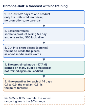
Text description of the diagram
Five boxes, one under the other. First, the last 512 days of one product: only the units sold, with no prices, promotions or calendar. Second, the values are scaled, so that a product selling 5 a day and one selling 500 a day look alike. Third, the series is cut into short pieces called patches; the model reads them as a text model reads words. Fourth, the pretrained model, with 47.7 million parameters, learned on many public time series and not trained again on Larkfield. Fifth, the output: nine quantiles for each of the 14 days, from 0.1 to 0.9; the median, 0.5, is the point forecast. A dashed box adds that there is no 0.05 or 0.95 quantile, so the widest range it gives is the 80% range.
A quantile is a level that the real value should fall below a given share of the time. The 0.9 quantile should be exceeded on about 1 day in 10. The 0.1 to 0.9 quantiles make an 80% range: about 8 real days in 10 should fall inside it. Module 7 is about ranges; here you need only this idea.
A tiny worked example: the parasol on 11 May 2025
Section titled “A tiny worked example: the parasol on 11 May 2025”Priya gives the model the parasol’s last 512 days up to Sunday 11 May 2025, at the start of the spring ramp. She asks for the 0.1, 0.5 and 0.9 quantiles of the next 14 days.
pipe = BaseChronosPipeline.from_pretrained("amazon/chronos-bolt-small", revision="772f3d25d38aec6d914c8949dab4462e2d46f5d8", device_map="cpu", torch_dtype=torch.float32)context = torch.tensor(parasol.loc[parasol["ds"] <= origin, "y"].to_numpy()[-512:], dtype=torch.float32)q, _ = pipe.predict_quantiles([context], prediction_length=14, quantile_levels=[0.1, 0.5, 0.9])revision fixes the exact version of the model, so the forecast does not change when its authors publish a new one. The output, added up over the 14 days:
{'q10': 96.7, 'q50': 181.8, 'q90': 309.7} | real: 216 | days inside the range: 12 of 14- Sold before the cut-off
- Forecast: median, and 0.1 and 0.9 quantiles (dashed)
- Sold in the 14 days
Text description of the chart
The chart shows the parasol’s daily sales for four weeks before 11 May 2025, rising from about 3 a day to 20. After the cut-off, three blue lines show the forecast for 14 days. The median is between 10.5 and 16.8 a day. The 0.1 quantile is between 4.5 and 10.1, and the 0.9 quantile between 19.0 and 26.6. The real sales are dots between 8 and 25 a day. Over the 14 days, the median adds up to 181.8 and the real sales to 216. 12 of the 14 days are inside the range.
Read it like Kenji. The median says 182 parasols; 216 were sold. The range says “between about 97 and 310”, and it held the real value on 12 of 14 days. A fair forecast for a model that never saw Larkfield before. Its median is too low here, because the spring ramp grows faster than it expects.
Larkfield: Chronos-Bolt in the course backtest
Section titled “Larkfield: Chronos-Bolt in the course backtest”Now the real test. The same 50 products, the same 13 origins, the same 14 days as every other row. 650 forecasts, no training:
method horizon MASE WAPE % bias % pinball fit s cost $Chronos-Bolt small, no training 14 0.784 38.7 -5.6 0.099 1.18 14750coverage of the 80% range: 0.789coverage of the 90% range: 0.789It wins on accuracy. MASE 0.784 and WAPE 38.7% are the best of the whole table: better than LightGBM (40.7%), ETS (41.3%) and every baseline. Its pinball loss, a score for a range that Module 7 explains, is also the best: 0.099 against 0.110 for ETS. Product by product, it has the lowest WAPE on 28 of the 50 products, and on the parasol (45.0%). Prediction is fast: 650 forecasts in about 2 seconds on a laptop CPU.
The course expected the opposite: that a model trained on other data would lose on Larkfield’s. It did not lose. Say this plainly. One honest caution: the Larkfield data is synthetic, made by a simple generator with clean weekly and yearly seasons. Real data with messy events may suit it less. That is a reason to backtest it on your data, not a reason to doubt this result.
Explore
Chronos-Bolt against the other methods, on the parasol
Predict first: Over all 13 origins, which method wins on the parasol: LightGBM or Chronos-Bolt?
- Sold in the 14 days
- 216
- Forecast for the 14 days
- 182
- WAPE at this origin
- 29.0%
- WAPE, all 13 origins
- 45.0%
At the origin 11 May 2025, Chronos-Bolt forecasts 182 units for the next 14 days. 216 were sold. Its WAPE here is 29.0%: it is too low. Over all 13 origins, Chronos-Bolt has a WAPE of 45.0%: number 1 of 6 methods. It beats the baseline, seasonal naive (66.1%).
- Units sold
- Forecast of the chosen method
- Baseline: seasonal naive
Show every method, ranked
| Rank | Method | Family | WAPE at this origin | WAPE, all 13 origins |
|---|---|---|---|---|
| 1 | Chronos-Bolt | foundation model | 29.0% | 45.0% |
| 2 | LightGBM (recursive) | machine learning | 33.3% | 49.3% |
| 3 | AutoARIMA | statistical | 26.6% | 62.6% |
| 4 | moving average (28 days) | baseline | 54.2% | 64.9% |
| 5 | ETS | statistical | 31.8% | 65.1% |
| 6 | seasonal naive | baseline | 38.9% | 66.1% |
Text description of the explorer
The explorer shows a chart of the parasol’s daily sales. The four weeks before the chosen origin are a grey line, and the 14 days after it are grey dots. The chosen method’s forecast is a blue line, and the seasonal naive forecast a dashed orange line. The controls choose the origin (13 April 2025 to 15 March 2026) and one of six methods. At the origin of 11 May 2025, 216 parasols were sold. Over all 13 origins, the WAPE of each method is: Chronos-Bolt 45.0%, LightGBM (recursive) 49.3%, AutoARIMA 62.6%, moving average (28 days) 64.9%, ETS 65.1% and seasonal naive 66.1%.
What it costs: read the rest of the row
Section titled “What it costs: read the rest of the row”A row has more columns than WAPE. Kenji reads all of them.
- Statistical method
- Machine learning
- Foundation model
Text description of the chart
Three panels. WAPE: ETS 41.3%, LightGBM recursive 40.7%, LightGBM direct 40.7%, Chronos-Bolt 38.7%. Bias: ETS +0.1%, LightGBM recursive +0.7%, LightGBM direct -0.6%, Chronos-Bolt -5.6%. Order cost: ETS 16,578 dollars, LightGBM recursive 14,749, LightGBM direct 13,711, Chronos-Bolt 14,750.
It forecasts too low
Section titled “It forecasts too low”The bias is −5.6%: over the whole backtest, the forecasts add up to 5.6% fewer units than were sold. The other methods are within 1.5% of zero. Too-low forecasts make too-small orders. Say Kenji orders the 14-day forecast added up. Then 56.6% of Chronos-Bolt’s orders run short, against 50.0% for ETS (measured in Module 7). So its order costs 14,750 dollars, 1,039 more than the direct LightGBM, although its WAPE is 2 points better.
It does not see the promotion calendar
Section titled “It does not see the promotion calendar”The model reads only the units sold. On the 154 promotion days, it forecast 1,060 units for 1,927 sold: -45%, as blind as ETS (-43.5%). LightGBM, which sees the flag, was +5.2%. Some versions of Chronos accept known inputs such as a promotion flag. The version in this course does not use them.
Its range stops at 80%
Section titled “Its range stops at 80%”Text description of the chart
Coverage of the 80% range: seasonal naive 87.7%, ETS 83.5%, AutoARIMA 83.0%, Chronos-Bolt 78.9%. Coverage of the 90% range: seasonal naive 92.9%, ETS 90.5%, AutoARIMA 90.2%, Chronos-Bolt 78.9%.
Its 80% range is a little narrow: it holds 78.9% of the real values instead of 80%. The real problem is the 90% range. Chronos-Bolt was trained to give only the quantiles 0.1 to 0.9. When you ask for 0.05 or 0.95, it warns and returns its 0.1 and 0.9 instead. So its “90% range” holds 78.9%, not 90%. Module 7 orders stock from a high quantile, so this matters.
It needs its own process, and memory
Section titled “It needs its own process, and memory”In the course’s tests on a Mac with Apple silicon, Chronos-Bolt and LightGBM in one Python process crashed with no error message. The crash came right after the model loaded. Both load their own copy of a library for parallel work (OpenMP). The course now runs Chronos in a separate process, and this lesson’s notebook does not import LightGBM. In production, that means a second job to run and watch.
The model has 47.7 million parameters. ETS keeps a handful of numbers per product. The download is about 190 MB, loading takes a few seconds, and the Python process peaked at about 895 MB of memory. On a CPU, it is fast, so the cost is not time. The cost is one more large dependency, pinned to one revision. Someone else trained it, on data that you have not seen.
When to use a foundation model, and when not
Section titled “When to use a foundation model, and when not”Use it:
- as a strong baseline that costs no training: if your own model cannot beat it in the backtest, you have learned something;
- for many series with little history, or a new business, where training your own model is hard;
- when a fast first forecast is worth more than the last few percent.
Do not use it, or not alone:
- when known future inputs drive the series (promotions, prices) and your set-up cannot pass them;
- when the decision needs a high quantile that the model does not give;
- when its bias costs money, as here; check the bias column, not only WAPE;
- when you cannot run, pin and watch one more large model.
Common mistake
A 90% range that is not there
Symptom: Tomás sets the safety stock from Chronos-Bolt’s 0.95 quantile, to run short on only about 1 order in 20. In the backtest, the real sales are above that quantile far more often than 1 time in 20.
Cause: Chronos-Bolt gives only the quantiles 0.1 to 0.9. For 0.05 and 0.95, it prints a warning and returns its 0.1 and 0.9. Its “90% range” holds 78.9% of the real values, the same as its 80% range.
Fix: read the warnings, and measure the coverage of every range you use in the backtest. Use a method whose range holds what it promises at that level, or widen the range from the backtest errors (Module 7).
Consequence in AI work: a model can return a number for any question you ask, even when it was not built to answer it. A range that looks right but holds less than it says turns into stock-outs that nobody planned for.
Guided practice: a foundation model in the notebook
Section titled “Guided practice: a foundation model in the notebook”- Open the notebook from the box Do this lesson in a notebook at the top of this page.
- Run the setup cells and the helper cell. The first cell can take 2 minutes, because it installs PyTorch.
- In section 1, predict the size of the model. Then run the cell. You see
parameters (millions): 47.7. - In section 2, predict if the median is above or below 216. Then run the cell. You see 181.8, and a chart of the range.
- In section 3, predict if the 90% range holds 90%. Then run the backtest. You see WAPE % 38.7, bias % −5.6 and two coverages of 0.789.
- In section 4, write your answer in the Your turn cell, then run the check cell.
Your turn: what the model does not see
Section titled “Your turn: what the model does not see”Before you run anything, predict: on promotion days, is Chronos-Bolt closer to ETS (−43.5%) or to LightGBM (+5.2%)? In the notebook, section 4, keep the promotion days of fc_chronos, compute their bias in % and put it in promo_bias_chronos.
Show the answer
p = fc_chronos.merge(sales[["unique_id", "ds", "on_promotion"]], on=["unique_id", "ds"])p = p[p["on_promotion"] == 1]promo_bias_chronos = round(float(100 * (p["yhat"].sum() - p["y"].sum()) / p["y"].sum()), 1)print(promo_bias_chronos, "% on", len(p), "promotion days")-45.0 % on 154 promotion daysChronos-Bolt is 45.0% too low on promotion days, like ETS. Both read only the past of the series. The best accuracy in total does not mean the best forecast on the days that matter most to Kenji.
Knowledge check
Section titled “Knowledge check”Check your understanding
Tomás says: 'The foundation model won, so we should replace everything with it.' Give two numbers that support him and three that do not.
Show the answer
For him: Chronos-Bolt has the best MASE (0.784) and WAPE (38.7%) of the course table, with no training. It has the lowest WAPE on 28 of the 50 products. Against him: its bias is −5.6%, so its orders run short more often. Its order costs 14,750 dollars, against 13,711 for the direct LightGBM. On the 154 promotion days, it is 45.0% too low, because it does not see the promotion calendar. And its 90% range holds only 78.9% of the real values, because it has no quantile beyond 0.1 and 0.9.
Does your answer have the main points of ours?
Sign in and enroll in the course to save your answers. Every check counts toward the certificate.
Check your understanding
What does 'zero-shot' mean for Chronos-Bolt, and what does it read from a Larkfield series in the course's set-up?
Show the answer
Zero-shot means that the model forecasts a series with no training on it, or on any Larkfield data. Its authors trained it once on many public time series. In the course’s set-up, it reads only the last 512 daily values of the units sold, scales them and cuts them into patches. It does not read prices, promotions or the calendar. It returns nine quantiles, 0.1 to 0.9, for each of the 14 days; the median is the point forecast.
Does your answer have the main points of ours?
Sign in and enroll in the course to save your answers. Every check counts toward the certificate.
Check your understanding
Name three costs of running Chronos-Bolt in Larkfield's weekly job that do not appear in the WAPE column.
Show the answer
It needs its own process: next to LightGBM in one Python process, it crashed with no error message. It is a large dependency, pinned to one revision. It has 47.7 million parameters, a download of about 190 MB and a memory peak of about 895 MB. And its range stops at the 0.1 and 0.9 quantiles. A decision that needs a 95% level gets the 90% one, unless someone reads the warning. Its bias of −5.6% also raises the order cost, although that one does appear in the table.
Does your answer have the main points of ours?
Sign in and enroll in the course to save your answers. Every check counts toward the certificate.
Recap
- Neural forecasters (N-BEATS, an RNN) learn from many series; they need large data, long training and tuning. The course did not run them.
- A foundation model is pretrained on many series and forecasts zero-shot. Chronos-Bolt small reads only the units sold and returns quantiles 0.1 to 0.9.
- On Larkfield it wins on accuracy: MASE 0.784 and WAPE 38.7%, best on 28 of 50 products. It makes 650 forecasts in about 2 seconds on a CPU.
- What it costs: a bias of −5.6%, so its order (14,750 dollars) is not the cheapest. It is −45.0% on promotion days and has no 90% range. It needs its own process and has 47.7 M parameters.
You now have simple, statistical, machine learning and foundation model rows in the table. The most accurate method is not the cheapest, and the cheapest is not the simplest. Next, you read the whole table for cost, speed and trust, and decide when a complex model is not worth it.