
Test like the future: backtesting
- Lesson 9
- 35 min
- Module 3: Baselines and honest testing
Where we are
We have four simple forecasts, but we have not yet tested them in a fair way. A random split lets the future leak into training. In this lesson, we test forecasts as the future will: a rolling-origin backtest with several cut-off dates. Think first of how you would test a weather forecaster.
Lesson 9 of 27 · Forecasting and Time Series: Predict What Comes NextTest like the future: backtesting
1. Forecasts serve decisions
2. Read a time series
3. Baselines and honest testing
4. Statistical forecasters
5. Machine learning forecasters
6. Hard series and many series
7. Uncertainty and the decision
8. Run a forecast in production
What you will be able to do
Test a forecast the way the future will test it. Cut the history at several past dates, forecast the days after each cut, and score all of them together. A random split lets the future into training, so the forecast looks better than it will be.
NotebookDo this lesson in a notebook
The notebook has every code cell, task and check of this lesson. It runs a backtest by hand, shows the course’s cut-off dates, tests the parasol at 13 dates, and compares a random split with an honest backtest. Its setup cells install the packages and download the Larkfield data, so it needs no local setup. About 30 minutes.
Colab and Kaggle open your own copy. They need a free Google or Kaggle account. Stuck? See the solution notebook.
Before you startWhat to know and to have ready
What you need to know
- The four naive forecasts and the helper
backtest.py, from Naive forecasts. - Yesterday’s sales predict today’s sales (autocorrelation), from Yesterday predicts today.
- Training and test sets: you judge a model on data that it did not learn from. See Train, validation and test sets in the machine learning course.
What you need on your computer
Nothing: the notebook runs in Colab or Kaggle. Section 4 of the notebook also installs scikit-learn.
Tested with Python 3.12, pandas 2.3.3, statsforecast 2.1.1 and scikit-learn 1.9.1, in Jupyter on macOS.
How to test a weather forecaster
Section titled “How to test a weather forecaster”You want to know if a weather forecaster is good, without waiting a whole year. So you find old newspapers. You take the forecast printed on a Monday, and you compare it with the weather of the days after that Monday.
Two rules make this test fair. First, the forecast must be printed before the weather happened. A “forecaster” who writes after he reads the weather report looks perfect and tells you nothing. Second, one newspaper is not enough. In one quiet, sunny week, every forecaster looks good. So you check many Mondays, spread over the whole year.
Forecasts at Larkfield need the same two rules. You met this test in short in Meet the Larkfield data, with two weather apps. This lesson shows what happens when the first rule breaks, then builds a test that keeps both.
The problem: a random split lets the future in
Section titled “The problem: a random split lets the future in”In the machine learning course, a model is often tested on a random split. You shuffle the rows and keep 20% of them as a test set. That works when the rows do not depend on each other. Sales do depend on each other: yesterday’s sales predict today’s. Yesterday predicts today showed a first case, a rule that read the neighbours of each test day.
Tomás tests a model in this way. It is a gradient boosting model, the kind of model that the machine learning course built. Its inputs are the sales of 1, 7 and 14 days before, the weekday and the promotion flag. He shuffles the days of the 50 products of the course and keeps 20% as a test:
d = sales.sort_values(["unique_id", "ds"]).copy()g = d.groupby("unique_id")["y"]d["lag1"], d["lag7"], d["lag14"] = g.shift(1), g.shift(7), g.shift(14)d["dow"] = d.ds.dt.dayofweekd = d.dropna()X, y = d[["lag1", "lag7", "lag14", "dow", "on_promotion"]], d["y"]Xtr, Xte, ytr, yte = train_test_split(X, y, test_size=0.2, random_state=35)model = HistGradientBoostingRegressor(random_state=35).fit(Xtr, ytr)print("random 20% test, WAPE %:", round(float(100 * np.abs(yte - model.predict(Xte)).sum() / yte.sum()), 1))shift(1) moves the sales down by one day, so each row gets the sales of the day before. These columns are called lags: lag1 is yesterday’s sales, lag7 the sales of one week before. The output:
random 20% test, WAPE %: 40.4A WAPE of 40.4% beats every naive forecast of the last lesson (the best was 43.5%). But look at what the random test allowed:
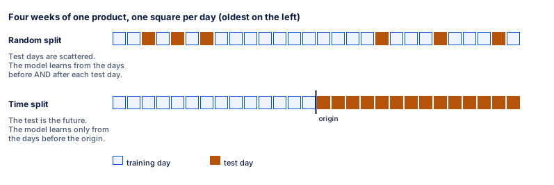
Text description of the diagram
The picture shows four weeks of one product as two rows of 28 squares, one per day. In the top row, the random split, six orange test squares sit among blue training squares. The model learns from the days around each test day. In the bottom row, the time split, 14 blue training days come first. A black line marks the origin, and 14 orange test days follow it.
A test day has training days on both sides of it, and its input lag1 is the real sales of the day before. On Kenji’s Monday, nobody knows what the parasol sells on the second Thursday. The test checks a situation that never happens.
Priya runs the honest version. At each of the course’s cut-off dates, the same kind of model learns only from the days up to that date. For a 14-day forecast, it may use only sales at least 14 days old: here, 14 and 21 days before.
honest 14-day backtest, WAPE %: 47.1Text description of the chart
A column chart with two columns on an axis from 0 to 60%. The random 20% test gives a WAPE of 40.4%. The honest 14-day backtest of the same kind of model gives 47.1%.
The model did not get worse. The test got honest, and now the model loses to a plain 28-day average (43.5%). This mistake is a form of leakage: information reaches the model from where it should not, here from the future.
The idea: a rolling-origin backtest
Section titled “The idea: a rolling-origin backtest”A backtest tests a forecast on the past, as if the past were the future. It copies the weather-forecaster test:
- Choose a cut-off date in the past. It is called the forecast origin, or origin for short. The forecast starts from it, and the method may see only the days up to it.
- Give the method every day up to the origin. It learns from them: this is its training window.
- Ask for a forecast of the next h days. h is the horizon.
- Compare the forecast with what was really sold in those days.
- Move the origin forward, and do it again. The method learns again at every origin, from the longer history. This is called a refit.
Because the origin moves forward step by step, this is a rolling-origin backtest. Many libraries call it time-series cross-validation. At the end, you score all the forecasts of all the origins together.
A tiny backtest
Section titled “A tiny backtest”A product sold these units on 12 days:
| Day | 1 | 2 | 3 | 4 | 5 | 6 | 7 | 8 | 9 | 10 | 11 | 12 |
|---|---|---|---|---|---|---|---|---|---|---|---|---|
| Sold | 4 | 6 | 5 | 7 | 9 | 6 | 8 | 10 | 7 | 9 | 12 | 8 |
We test the naive forecast (the last value) with a horizon of 2 days, at three origins: day 6, day 8 and day 10.
| Origin | Sees days | Last value | Forecast days | Forecast | Sold | Miss |
|---|---|---|---|---|---|---|
| Day 6 | 1 to 6 | 6 | 7, 8 | 6, 6 | 8, 10 | 2, 4 |
| Day 8 | 1 to 8 | 10 | 9, 10 | 10, 10 | 7, 9 | 3, 1 |
| Day 10 | 1 to 10 | 9 | 11, 12 | 9, 9 | 12, 8 | 3, 1 |
The misses add up to 2 + 4 + 3 + 1 + 3 + 1 = 14 units. The six days sold 54 units. So the WAPE is 14 ÷ 54 = 25.9%. bt.backtest() does the same work for any forecaster:
tiny = pd.DataFrame({"unique_id": "shop", "ds": pd.date_range("2025-06-01", periods=12, freq="D"), "y": [4, 6, 5, 7, 9, 6, 8, 10, 7, 9, 12, 8]})cuts = [pd.Timestamp("2025-06-06"), pd.Timestamp("2025-06-08"), pd.Timestamp("2025-06-10")]fc = bt.backtest(tiny, bt.naive, h=2, origins=cuts)fc["miss"] = (fc["y"] - fc["yhat"]).abs()print(fc[["origin", "step", "ds", "y", "yhat", "miss"]].to_string(index=False))print("misses added up:", fc["miss"].sum(), "| units sold:", fc["y"].sum(), "| WAPE %:", round(100 * fc["miss"].sum() / fc["y"].sum(), 1))The output:
origin step ds y yhat miss2025-06-06 1 2025-06-07 8 6 22025-06-06 2 2025-06-08 10 6 42025-06-08 1 2025-06-09 7 10 32025-06-08 2 2025-06-10 9 10 12025-06-10 1 2025-06-11 12 9 32025-06-10 2 2025-06-12 8 9 1misses added up: 14 | units sold: 54 | WAPE %: 25.9step counts the days after the origin. Every row is a forecast made without its real value, as in real use.
The course backtest
Section titled “The course backtest”Every module of this course uses the same backtest, so that every row of the backtest table is comparable. It has 13 origins, 28 days apart; the last one is Sunday 15 March 2026. At each origin, a method forecasts the next 14 days.

Text description of the diagram
The diagram has 13 rows on one time axis, from April 2024 to March 2026. Each row is one origin, from 13 April 2025 (top) to 15 March 2026 (bottom). In every row, a blue bar runs from 1 April 2024 to the origin: the training window. A short orange bar covers the next 14 days: the test. Each row’s bars are 28 days longer and later than the row above. The last orange bar ends on 29 March 2026.
print(len(ORIGINS), "origins:", [o.date().isoformat() for o in ORIGINS])start = pd.Timestamp("2024-04-01")for o in [ORIGINS[0], ORIGINS[-1]]: print(f"origin {o.date()}: trains on {(o - start).days + 1} days, tests {o.date() + pd.Timedelta(days=1)} " f"to {o.date() + pd.Timedelta(days=14)}")13 origins: ['2025-04-13', '2025-05-11', '2025-06-08', '2025-07-06', '2025-08-03', '2025-08-31', '2025-09-28', '2025-10-26', '2025-11-23', '2025-12-21', '2026-01-18', '2026-02-15', '2026-03-15']origin 2025-04-13: trains on 378 days, tests 2025-04-14 to 2025-04-27origin 2026-03-15: trains on 714 days, tests 2026-03-16 to 2026-03-29Each choice has a reason:
- 14 days ahead, because Kenji orders on Mondays and the order must cover two weeks. The horizon comes from the decision, as in Frame the forecast.
- 28 days apart, so the test windows never overlap. Thirteen of them cover a whole year: the spring ramp, the summer peak, Black Friday, Christmas and the quiet winter.
- The first origin after more than a year of history, so that a method that needs a full yearly season can run at every origin.
- A refit at every origin, because in real use the method learns again from the newest data every week.
- Origins on Sundays, because Kenji’s order on Monday uses the sales up to Sunday.
The weeks after 29 March 2026 are the hidden future. The course keeps them back for the final assignment, so that one honest test stays unused until the end.
The horizon decides the gap
Section titled “The horizon decides the gap”On Monday, Kenji knows the sales up to Sunday. For the second Sunday of the order, the newest known sale is 14 days old. So a model with one set of inputs for the whole order may use only what is at least 14 days old. This gap is set by the horizon of the decision. Tomás’s lag1 broke it; the honest model used lag14 and lag21. Module 5 shows two more ways to build a model that keeps the gap: a recursive forecast and one model per day ahead.
Larkfield: the parasol at 13 origins
Section titled “Larkfield: the parasol at 13 origins”Priya backtests the seasonal naive forecast (the same weekday last week) on the parasol alone, and scores each origin on its own:
parasol = load_sales(["P025"])fc = bt.backtest(parasol, bt.seasonal_naive(7), h=14, origins=ORIGINS)per_origin = fc.groupby("origin").apply(lambda g: 100 * (g["y"] - g["yhat"]).abs().sum() / g["y"].sum())print(per_origin.round(1).to_string())print("all 13 origins together:", bt.score(fc, parasol, "seasonal naive", season=7)["WAPE %"])origin2025-04-13 55.62025-05-11 38.92025-06-08 74.32025-07-06 98.92025-08-03 49.42025-08-31 35.42025-09-28 69.92025-10-26 176.92025-11-23 157.12025-12-21 154.52026-01-18 100.02026-02-15 118.22026-03-15 116.7all 13 origins together: 66.1Text description of the chart
The chart has 13 dots, one per origin, joined by a line. From April to September 2025, the WAPE stays between 35.4% (31 August) and 98.9% (6 July, the week after the heat wave). From October 2025 to March 2026, it is 100% or more, with the highest value, 176.9%, on 26 October. The WAPE over all 13 origins together is 66.1%.
A WAPE above 100% means that the misses add up to more than the units sold. In winter, the parasol sells almost nothing, so a small miss is a large share. One origin tells you more about its date than about the method. Thirteen origins over a year cover every season.
Which method wins on the parasol?
Section titled “Which method wins on the parasol?”The explorer below has the same 13 origins and eight methods. Four of them come later in the course; treat them as black boxes for now:
- ETS and AutoARIMA: statistical methods that fit a model to each series (Module 4).
- LightGBM (recursive): one gradient boosting model for all products (Module 5).
- Chronos-Bolt: a pretrained model that forecasts with no training on Larkfield data (Module 5).
Move the origin along the year and switch between methods. The dashed line is the seasonal naive baseline.
Explore
The parasol in the course backtest
Predict first: Which method wins on the parasol over 14 days, scored on all 13 origins?
- Sold in the 14 days
- 101
- Forecast for the 14 days
- 118
- WAPE at this origin
- 74.3%
- WAPE, all 13 origins
- 66.1%
At the origin 8 Jun 2025, seasonal naive forecasts 118 units for the next 14 days. 101 were sold. Its WAPE here is 74.3%: it is too high. Over all 13 origins, seasonal naive has a WAPE of 66.1%: number 6 of 8 methods.
- Units sold
- Forecast of the chosen method
- Baseline: seasonal naive
Show every method, ranked
| Rank | Method | Family | WAPE at this origin | WAPE, all 13 origins |
|---|---|---|---|---|
| 1 | Chronos-Bolt | foundation model | 58.1% | 45.0% |
| 2 | LightGBM (recursive) | machine learning | 44.8% | 49.3% |
| 3 | AutoARIMA | statistical | 51.7% | 62.6% |
| 4 | moving average (28 days) | baseline | 101.3% | 64.9% |
| 5 | ETS | statistical | 45.5% | 65.1% |
| 6 | seasonal naive | baseline | 74.3% | 66.1% |
| 7 | naive | baseline | 50.5% | 90.9% |
| 8 | drift | baseline | 50.3% | 92.5% |
Text description of the explorer
The explorer shows the parasol’s daily sales. The four weeks before the chosen origin are a grey line, and the 14 days after it are grey dots. The chosen method’s forecast is a blue line, and the seasonal naive forecast a dashed orange line. A strip above shows the 13 test windows. The controls choose the origin and one of eight methods. The readout shows the units sold, the forecast, the WAPE at this origin and over all 13 origins. At the origin of 8 June 2025, 101 parasols were sold; the seasonal naive forecast was 118, a WAPE of 74.3% at this origin. Over all 13 origins, the WAPE of each method is: Chronos-Bolt 45.0%, LightGBM (recursive) 49.3%, AutoARIMA 62.6%, moving average (28 days) 64.9%, ETS 65.1%, seasonal naive 66.1%, naive 90.9% and drift 92.5%.
On the parasol, Chronos-Bolt wins with a WAPE of 45.0%, then LightGBM with 49.3%. Both are far ahead of the seasonal naive baseline (66.1%). ETS and AutoARIMA beat it only a little, and the 28-day moving average does as well as ETS.
This is one product, and on others the order changes: the seasonal naive forecast beats LightGBM on 3 of the 50. What matters here is that the comparison is fair: the same origins, horizon and days for every method.
When to use a backtest, and what it costs
Section titled “When to use a backtest, and what it costs”Use a rolling-origin backtest for every forecast that you compare or report. Keep it the same for every method, or the rows of the table do not compare.
It has costs:
- Time. A refit at every origin means 13 fits per series instead of one. AutoARIMA in Module 4 took about 1,000 seconds for 50 products and 13 origins.
- History. Every origin needs history before it. With a few months of data, you get fewer origins, and more chance in the score.
- Many looks. If you try 30 versions of a method and keep the best backtest score, part of its lead is luck. The machine learning course showed the same with a validation set. That is why the hidden quarter stays unused until the final assignment.
When the horizon or the cost of a refit is very large, you can refit less often: for example, every fourth origin. bt.backtest() has a refit_every argument for that. Say so next to the score.
Common mistake
One cut-off date
Symptom: Tomás tests the seasonal naive forecast on the parasol at one origin, 31 August 2025. He gets a WAPE of 35.4% and writes: “Same weekday last week works well for parasols.” Kenji tries it in late October and misses more than all the units sold (176.9%).
Cause: one origin is one window of 14 days. Its score depends on the season and on luck as much as on the method. Late August is calm and steady for parasols; late October has very few sales.
Fix: backtest at several origins spread over a whole year, and report the score of all of them together: 66.1% for the parasol. Look at the scores per origin too.
Consequence in AI work: a single test window makes a forecast look better or worse than it is, by chance. Decisions based on it, such as a method for a whole category, fail in the next season.
Guided practice: a backtest in the notebook
Section titled “Guided practice: a backtest in the notebook”- Open the notebook from the box Do this lesson in a notebook at the top of this page.
- Run the setup cells and the helper cell. The data cell ends with the
Ready:line. - In section 1, predict at which origin the forecast misses most. Then run the cell. You see
WAPE %: 25.9. - In section 2, run the cell. You see
13 originsand the training days of the first and last origin. - In section 3, predict if the WAPE is the same at every origin. Then run the cell. You see 13 values and
66.1for all of them together. - In section 4, predict which test gives the lower WAPE. Then run the random split. You see
40.4. - Run the honest backtest. You see
47.1. - In section 5, write your answer in the Your turn cell, then run the check cell.
Your turn: a shorter horizon
Section titled “Your turn: a shorter horizon”bt.score() has a horizon= argument that keeps only the first days after each origin. Before you run it, predict: is the seasonal naive forecast better or worse on the first 7 days than on all 14? In the notebook, section 5, score fc_sn with horizon=7 and put its WAPE % in wape_h7.
Show the answer
wape_h7 = bt.score(fc_sn, sales, "seasonal naive", season=7, horizon=7)["WAPE %"]print(wape_h7)49.8The first week is easier: 49.8% against 51.3% for all 14 days. In the second week, the forecast repeats a week that is already 8 to 14 days old. A forecast gets worse further ahead, so score it at the horizon of the decision. A 7-day score would make the method look better than it will be for Kenji’s 14-day order.
Knowledge check
Section titled “Knowledge check”Check your understanding
Explain with Larkfield's numbers how a random split made a model look better than it is, and what the honest test showed.
Show the answer
On a random 20% test, a gradient boosting model with the sales of 1, 7 and 14 days before missed 40.4% of the units. That beats every baseline. But the random test let the future in. Each test day had training days on both sides. Its input lag1 was yesterday’s real sales, which Kenji does not know for most days of a 14-day order. In an honest 14-day backtest, the same kind of model may use only sales at least 14 days old. It missed 47.1%, worse than the 28-day moving average (43.5%).
Does your answer have the main points of ours?
Sign in and enroll in the course to save your answers. Every check counts toward the certificate.
Check your understanding
Name the parts of a rolling-origin backtest, and give the values of the course backtest.
Show the answer
- Origin: the cut-off date; the method sees only the days up to it. The course uses 13 origins, from 13 April 2025 to 15 March 2026, 28 days apart.
- Training window: every day from 1 April 2024 to the origin.
- Horizon: the days forecast after each origin: 14, the length of Kenji’s order.
- Refit: the method learns again at every origin.
- Score: all forecasts of all origins together, for example the WAPE of all 9,100 forecast days of the 50 products.
Does your answer have the main points of ours?
Sign in and enroll in the course to save your answers. Every check counts toward the certificate.
Check your understanding
Predict: Grace plans the help-desk roster one week ahead, hour by hour. What horizon should the ticket backtest use, and which lags can a model use?
Show the answer
The horizon is one week: 168 hours, the time the roster must cover. On the day Grace makes the roster, she knows the tickets up to that day. So for the last hour of the week, the newest known value is 168 hours old. A model that forecasts every hour of the week with one set of inputs may use only lags of 168 hours or more. A lag of 1 hour or 24 hours would let the future in, as lag1 did in Tomás’s random test. The course’s ticket backtest uses this horizon.
Does your answer have the main points of ours?
Sign in and enroll in the course to save your answers. Every check counts toward the certificate.
Recap
- A random split lets the future into training. The same kind of model missed 40.4% on a random test and 47.1% on an honest backtest.
- A rolling-origin backtest cuts the history at several origins, forecasts the horizon after each, and scores everything together.
- The course backtest: 13 origins, 28 days apart, from 13 April 2025 to 15 March 2026; a 14-day horizon (Kenji’s order); a refit at every origin.
- The horizon decides the gap: a 14-day forecast may use only what is at least 14 days old.
- One origin is not a test: the parasol’s seasonal naive WAPE moved from 35.4% to 176.9% with the date. On all 13 origins, Chronos-Bolt wins on the parasol (45.0%), then LightGBM (49.3%).
You can now test any forecast fairly. But we have scored with WAPE only, and a single number can hide what matters to Kenji. Next, you compare the error measures and see where each one breaks.