
Rules and colour histograms
- Lesson 5
- 40 min
- Module 2: Baselines and pretrained classifiers
Where we are
We have the images, the splits and an empty comparison table. It is tempting to start with a big model. In this lesson, we start with the simplest methods instead: rules on colour and size, and a colour histogram with nearest neighbours. First, a worker in the returns warehouse sorts parcels by eye.
Lesson 5 of 30 · Vision AI: See, Count and InspectRules and colour histograms
1. Seeing is a business problem
2. Baselines and pretrained classifiers
3. Embeddings, CLIP and few labels
4. Detect and count
6. Inspect for defects
7. Match, search and describe
8. Run vision in production
What you will be able to do
Build the two simplest image classifiers, a hand-written rule and a colour histogram with nearest neighbours, and measure them on the catalogue. Every later method must beat them, and you must know where they are good enough.
NotebookDo this lesson in a notebook
The notebook has every code cell, task and check of this lesson. Its setup cells install the packages and download the catalogue photos (about 9 MB, as zip files). It needs no account and no key. About 25 minutes.
Colab and Kaggle open your own copy. They need a free Google or Kaggle account. Stuck? See the solution notebook.
Before you startWhat to know and to have ready
What you need to know
- Pixels, channels and the HSV colour space, from Images are numbers.
- The catalogue, its splits and the comparison table, from Meet the Larkfield images.
- Accuracy and recall, from Classification metrics in Machine Learning: From Problem to Reliable Model.
What you need on your computer
- The notebook route: a browser, and Colab or Kaggle. Nothing to install.
- The project route: the
larkvisionfolder of the last lesson, besidenextia-learning-labs, with its virtual environment. It is at the snapshotstartnow. In this lesson it moves toend-of-m02.
Tested with Python 3.12.13 on macOS. The Windows commands were not tested.
A worker sorts parcels by eye
Section titled “A worker sorts parcels by eye”A new worker starts in Larkfield’s returns warehouse. On her first day, she sorts returned parcels into bins: candles, plant pots, cushions and the rest. Nobody gives her a list of rules. After an hour, she has her own: “Small and white is a candle. Green leaves on top is a plant pot. Soft and light is a cushion.”
Her rules work in her warehouse, under her lamps, on her table. Move her to another warehouse with yellow light and a dark table, and some rules stop working. “White” now looks cream. This lesson builds her two kinds of shortcut as code. The first is a rule that a person writes. The second is a colour histogram, which compares colours with known photos.
A rule that a person writes
Section titled “A rule that a person writes”Priya looked at 20 catalogue photos and wrote four rules in Python. Each rule reads simple numbers from the photo, shrunk to 64 × 64 pixels:
- A bright centre on a dark border is a candle (a flame in a dark room).
- More than 12% of green pixels is a plant pot (leaves).
- A very light photo (mean brightness above 170 of 255) is a cushion.
- Everything else is a chair, the largest class.
Section 2 of the notebook runs this rule on the 160 test photos:
pred = [rule("data/" + f) for f in test["file"]]s = cp.classification_scores(list(test["label"]), pred, CLASSES)print("accuracy", s["accuracy"], "| worst class", s["worst_class"], s["worst_recall"])accuracy 0.269 | worst class bowl 0.0{'bowl': 0.0, 'candle': 0.3, 'chair': 0.8, 'cushion': 0.4, 'lamp': 0.0, 'mug': 0.0, 'plant_pot': 0.65, 'vase': 0.0}The rule is right on 26.9% of the photos. A random guess among eight classes is right on 12.5%, so the rule learned something. The chart shows where:
Text description of the chart
A column chart with eight columns, one per category, on an axis from 0 to 1. Bowl 0, candle 0.30, chair 0.80, cushion 0.40, lamp 0, mug 0, plant pot 0.65 and vase 0. The four categories without a rule are never right.
Recall is the share of a category’s photos that the method finds. Chair has a high recall (0.80) only because “everything else” goes to chair. Bowl, lamp, mug and vase have no rule, so they are never right.
The rules also fail where they do apply. Most catalogue candles stand on a white table in daylight, not in a dark room. So the candle rule finds only 6 of the 20 test candles. To fix it, Priya would add a fifth rule, then a sixth. Each new rule breaks an old one somewhere. This is the main problem of rules: a person must think of every case, and photos have too many cases.
A colour histogram
Section titled “A colour histogram”The worker has a second shortcut. She does not describe a candle in words. She remembers how candles look, and compares. A computer can do a simple version of this: it compares the colours of two photos.
A photo has 65,536 pixels at 256 × 256. Comparing them one by one fails: move the product a little, and every pixel changes. So we count instead. A colour histogram counts how many pixels have each colour. The word “histogram” means a count of values put into groups, called bins. The counts do not depend on where the product is in the photo.
A tiny worked example
Section titled “A tiny worked example”The picture below is a tiny image of 4 × 4 = 16 pixels, made by hand for this example. G is green, B is brown and W is white.
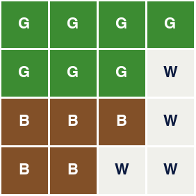
Text description of the diagram
The grid has four rows of four squares. The first row is four green squares. The second row is three green squares and one white. The third row is three brown squares and one white. The fourth row is two brown squares and two white. In all, 7 green, 5 brown and 4 white pixels.
Count each colour, and divide by 16 so that photos of any size compare fairly:
| Bin | Pixels | Share |
|---|---|---|
| Green | 7 | 7 / 16 = 0.44 |
| Brown | 5 | 5 / 16 = 0.31 |
| White | 4 | 4 / 16 = 0.25 |
The three shares are the histogram of this tiny image: (0.44, 0.31, 0.25). Swap two pixels, and the histogram stays the same.
Two real products
Section titled “Two real products”Real photos have thousands of colours, so the bins are ranges of colour. The picture below uses nine bins. Eight bins are ranges of hue, the colour’s place on the colour wheel, for clear colours. One bin holds grey, white and black pixels.

Text description of the diagram
Two photos, each with a column chart of nine bars. The candle photo is a flame on a black background. Its histogram: red-orange 16%, pink 3%, and 80% grey, white or black; the other bars are 0. The plant pot photo shows green leaves. Its histogram: red-orange 7%, yellow 20%, green 25%, and 48% grey, white or black. The two histograms look very different, so a computer can tell these two photos apart by colour alone.
The picture simplifies. The course’s method uses 128 bins: 8 ranges of hue × 4 of saturation × 4 of value. Saturation is how strong the colour is, and value is how bright it is. These are the three parts of the HSV colour space. The code takes the square root of each share. This makes the distances between histograms more fair (the notebook explains it in one line).
Nearest neighbours: compare with photos you know
Section titled “Nearest neighbours: compare with photos you know”Now we have one histogram per photo. How do we turn it into a label? The worker compares a new parcel with parcels she remembers. The method does the same. It finds the training photos whose histograms are closest to the new photo’s histogram, and takes their label. This is the k-nearest-neighbours method, or k-NN: k is the number of close photos that vote.
“Close” means a short distance. Take the differences between two histograms, bin by bin. Square them, add them up, and take the square root. Here is the tiny image against three training images with three bins. The numbers are made up for the example:
| Training image | Green | Brown | White | Distance to (0.44, 0.31, 0.25) |
|---|---|---|---|---|
| Plant pot | 0.50 | 0.30 | 0.20 | √(0.06² + 0.01² + 0.05²) = 0.08 |
| Bowl | 0.10 | 0.60 | 0.30 | √(0.34² + 0.29² + 0.05²) = 0.45 |
| Cushion | 0.05 | 0.05 | 0.90 | √(0.39² + 0.26² + 0.65²) = 0.80 |
With k = 1, the closest image votes alone: the tiny image is a plant pot. With k = 3, all three vote, one vote each. Then there is no majority, and the method breaks the tie with a fixed rule. A larger k is calmer, because one odd neighbour does not decide. But a small class has fewer photos to vote with. Keep this in mind for the candle.
The histogram on the Larkfield catalogue
Section titled “The histogram on the Larkfield catalogue”Sections 3 and 4 of the notebook compute the histogram of every photo and train k-NN with k = 5:
knn = KNeighborsClassifier(5, n_jobs=1).fit(Xtr, train["label"])for name, X, y in (("catalogue test", Xte, test["label"]), ("new studio", Xst, studio["label"])): s = cp.classification_scores(list(y), list(knn.predict(X)), CLASSES) print(f"{name:15s} accuracy {s['accuracy']} worst {s['worst_class']} {s['worst_recall']}")catalogue test accuracy 0.263 worst vase 0.05new studio accuracy 0.225 worst cushion 0.0The histogram reaches 0.263, about the same as the rule. It finds only one test vase of 20. Look at one vase, and the five training photos that the method found closest:

Text description of the diagram
Six photos in a row. The first is the test photo: a round brown vase with dry flowers. The next five are its nearest training photos by colour histogram, each with its label and its distance: a wooden chair at 0.48, a brown leather armchair at 0.56, a plant pot with red flowers at 0.57, a white bowl on a brown wooden table at 0.60 and a mug of tea on a brown table at 0.62. All six photos are mostly brown and white. None of the five is a vase, so the method answers “chair”.
Every neighbour is brown and white, like the vase. The method did exactly what it promised: it found the same colours. But colour does not tell a vase from a chair. The closest training vase is at a distance of 0.691, far behind the fifth neighbour. In the catalogue, products of every category come in every colour.
How many neighbours?
Section titled “How many neighbours?”Your turn in the notebook (section 5) tries k = 1 and k = 15. The course team’s runs:
| k | Accuracy (test) | Candle recall | Accuracy (new studio) |
|---|---|---|---|
| 1 | 0.275 | 0.15 | 0.269 |
| 5 | 0.263 | 0.1 | 0.225 |
| 15 | 0.325 | 0 | 0.275 |
With k = 15, the accuracy rises to 0.325, but the candle recall falls to 0. Candle has only 15 training photos (a problem we planted). With 15 voters, the large classes nearly always win the vote. A better overall number can hide a worse result for the class that matters. This is why the comparison table has a worst column.
Add the baseline to your project
Section titled “Add the baseline to your project”The project gets the same two methods as a command, vision baseline. You copy the new files from the snapshot end-of-m02. Before you copy, check the place: you must be in your larkvision folder, with the virtual environment active.
-
Open a terminal and go to your
larkvisionfolder. Activate the virtual environment:source .venv/bin/activateon macOS and Linux,.venv\Scripts\Activate.ps1on Windows. -
If this is a new terminal, set
LARKVISION_DATAagain. It lives only in the terminal where you set it. The command is step 5 of The project on your computer. -
Copy the files of this module from the snapshot:
Terminal window S=../nextia-learning-labs/C42/snapshots/end-of-m02for f in larkvision/features.py larkvision/commands/baseline.py tests/test_baseline.py requirements.txt README.md; do cp "$S/$f" "$f"; doneTerminal window $S = "..\nextia-learning-labs\C42\snapshots\end-of-m02"foreach ($f in 'larkvision\features.py', 'larkvision\commands\baseline.py', 'tests\test_baseline.py', 'requirements.txt', 'README.md') { Copy-Item "$S\$f" $f } -
Install the new packages.
requirements.txtnow adds SciPy, scikit-learn and scikit-image:Terminal window pip install -r requirements.txt -
Run the tests. You see
11 passed. The two new tests train both methods on a tiny fake data folder:Terminal window python -m pytest -q -
Run the colour histogram on the catalogue. It takes about 2 seconds:
Terminal window vision baseline --method histogram
The output of step 6:
colour histogram + 5-NN, catalogue test: accuracy 0.263; worst class vase (recall 0.05); 1.0 ms per photocolour histogram + 5-NN, new studio: accuracy 0.225; worst class cushion (recall 0.00); 0.9 ms per photoAdded to outputs/table.json. See it with: vision compare --task catalogueThe accuracies are the notebook’s. Your milliseconds differ: they depend on your computer. larkvision/features.py holds the function colour_histogram, the same code as in the notebook. vision baseline --k 15 tries another k. Now your project matches the snapshot end-of-m02, except for your own outputs folder.
Where a colour rule wins
Section titled “Where a colour rule wins”So far, colour lost. But the catalogue is the hard case for colour. Its photos come from thousands of cameras, rooms and lights. Now take the opposite case: one camera, one light, one table, one product.
Hamid’s returns photos are like that. Every tea light is photographed from above, on the same background, under the same light. There, a colour rule has a real chance. The course team wrote one: count the pixels on the wax that are much darker or more coloured than the wax around them. Many odd pixels means a damaged candle. The count of odd pixels is the photo’s score. Two lines on that score decide. At or above the check line, a person looks. At or above the fail line, the item goes to the outlet. Both lines were chosen on the validation photos, then measured once on the test photos. Set the line with the warehouse shows how to choose them.
- Reference
- The colour rule
- The floor
Text description of the chart
A column chart with four columns, in dollars a day for 600 returns. No check: 2,229.4. A person checks 100 random returns: 1,907.8. The colour rule: 1,779.4. A perfect inspector: 24.8. The colour rule is the cheapest of the first three, and far from perfect.
The rule costs 1,779 dollars a day. That is less than sending every return back on sale (2,229), and less than 100 random checks (1,908). It sends about 91 returns a day to a person, inside Hamid’s budget of 100. It marks no good candle as damaged. It needs no labelled photo, no model file, and 2.09 ms per photo.
But it is honest to show the rest too. The rule found only 4 of the 18 damaged test candles. It misses a chunk of wax that is gone, because the hole has the same colour as the wax. About 39 damaged items a day would still go back on sale. Later modules reach 369 dollars a day with models that compare small parts of each photo.
When to use rules and histograms
Section titled “When to use rules and histograms”- Use them when the camera, the light and the background are fixed, and the classes differ in colour or brightness. A sorting line with one product of each colour is a good case. Also use them as the first row of a comparison table. They take minutes to build and run in about 1 ms on any computer.
- Do not use them when photos come from many cameras or lights, as in the catalogue. Also avoid them when two classes share colours (brown vases and brown chairs).
- What they cost: almost nothing to run. The real cost is a person’s time to write and repair rules. And if the light changes, every rule and every histogram changes too.
Common mistake
The light changes, and the histogram breaks
Symptom: the same products, photographed in Larkfield’s new studio with warmer light, lose accuracy. The histogram falls from 0.263 to 0.225. Cushion recall falls to 0.00: no cushion is found.
Cause: the new studio is a problem we planted: the same 160 test photos, with warmer light added by code. Warm light moves white and grey pixels toward yellow and orange. The colour bins of the histogram change, but the products do not.
Fix: keep the light fixed where you can. A camera with fixed white balance and a lamp that does not change is a real fix. If the light must change, measure again on photos under the new light before you trust the method. Module 8 tries a simple colour correction, and measures it.
Consequence in AI work: a method that reads colour depends on the light. It can pass every test in one room and fail in the next one, with no error message.
Your turn: how many neighbours?
Section titled “Your turn: how many neighbours?”Section 5 of the notebook has a task with two check cells.
- Train the nearest-neighbour classifier with
k = 1, on the same histograms. - Put its test accuracy in
acc_k1, ascp.classification_scoresgives it. - Do the same with
k = 15, and put the result inacc_k15. - Run the two check cells. Each one prints
Check passedwhen your number is right. - Look at the candle recall of k = 15. Write one sentence on why it is 0.
Show the answer
acc_k1 = cp.classification_scores(list(test["label"]), list(KNeighborsClassifier(1, n_jobs=1).fit(Xtr, train["label"]).predict(Xte)))["accuracy"]acc_k15 = cp.classification_scores(list(test["label"]), list(KNeighborsClassifier(15, n_jobs=1).fit(Xtr, train["label"]).predict(Xte)))["accuracy"]print(acc_k1, acc_k15)0.275 0.325With k = 15, a test candle needs 8 candle votes among its 15 neighbours. But all the training photos hold only 15 candles. The large classes win nearly every vote, so no candle is found.
Knowledge check
Section titled “Knowledge check”Check your understanding
Priya's rule gets 0.269 and the colour histogram 0.263 on the catalogue. Why is a hand-written rule hard to improve, even for a person who looks at many photos?
Show the answer
A person must think of every case, and photos have too many cases. The candle rule expects a dark room, but most catalogue candles are on a white table in daylight. Each new rule fixes some photos and breaks others. Four classes (bowl, lamp, mug, vase) have no rule at all, so their recall is 0.
Does your answer have the main points of ours?
Sign in and enroll in the course to save your answers. Every check counts toward the certificate.
Check your understanding
A test vase is brown and white. Its five nearest training photos by colour histogram are two chairs, a plant pot, a bowl and a mug. Is the method broken? What does this tell you?
Show the answer
The method is not broken: it found the photos with the closest colours, as promised. The problem is the feature. In the catalogue, every category comes in many colours, and many products are brown, white or grey. Colour alone cannot tell a vase from a chair. A feature that describes shape is needed, which is the next lesson.
Does your answer have the main points of ours?
Sign in and enroll in the course to save your answers. Every check counts toward the certificate.
Check your understanding
Hamid asks: 'Should we use a colour rule for the returns?' Answer with numbers from this lesson, and say what you would watch.
Show the answer
It is a cheap first step, and better than no check. On the test photos, the rule costs about 1,779 dollars a day. No check costs 2,229, and 100 random checks cost 1,908. It sends about 91 returns a day to a person, inside the budget of 100. It needs no labels and about 2 ms a photo. It works only because the camera, light and background are fixed. It also finds only 4 of 18 damaged candles, so do not stop there. Watch the light: if the camera or the lamp changes, measure again before you trust it.
Does your answer have the main points of ours?
Sign in and enroll in the course to save your answers. Every check counts toward the certificate.
Recap
- A rule written by a person reaches 0.269 on the catalogue. It can never be right for bowl, lamp, mug or vase, because they have no rule.
- A colour histogram counts pixels in colour bins. k-NN gives a photo the label of its closest training photos. It reaches 0.263, and 0.225 under the warmer studio light.
- A larger k gave 0.325, but no candle at all: a better overall number can hide the worst class.
- Your project now has
vision baseline --method histogramand 11 tests, as the snapshotend-of-m02. - Colour wins with a fixed camera and fixed light. A colour rule on the returns costs 1,779 dollars a day, against 2,229 with no check.
You can now build and measure a colour method. But the histogram knows nothing about shape: a brown vase and a brown chair look the same to it. Next, you describe shapes with hand-made edge features, and see what that adds.
Next: Hand-made features